DOX Tools
October 19, 2019
The design of experiments (DOE, DOX, or experimental design) is the design of any task that aims to describe or explain the variation of information under conditions that are hypothesized to reflect the variation[1]. Montgomery specifies [2] that experimental design is a tool for engineers and scientists to use for product design and development as well as process development and improvement.
Statistical software are specialized computer programs for analysis in statistics. In general, statistical software is needed to calculate necessary numerical values when you analyze the subject in DOX. There are various statistical software tools[3] you can use in your study. Some authors prefer to use open-source, public domain, or freeware tools in their DOX books while others use proprietary software or add-ons.
Recommendations
You can see couple of products in below table which I prefer to use in my studies.
| Products - Open Source | Help |
|---|---|
| GNU Octave Wiki Gretl User's Guide R packages for DOX DOX packages for Python |
|
| Products - Proprietary | Help |
| EViews Help Maple Help Minitab Support Statistical Data Analysis Mathworks Documentation SPSS Help |
An Example
Example from Montgomery[2], p.25.
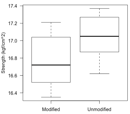
An engineer is studying the formulation of a Portland cement mortar. He has added a polymer latex emulsion during mixing to determine if this impacts the curing time and tension bond strength of the mortar. The experimenter prepared 10 samples of the original formulation and 10 samples of the modified formulation.
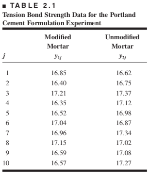
Figure: Screenshot of the Table 2.1. in Montgomery's book[2], p.26.
Solution in R Language
See Appendix: R Code.
> t.test(y1,y2,var.equal=TRUE)

	Two Sample t-test

data:  y1 and y2
t = -2.1869, df = 18, p-value = 0.0422
alternative hypothesis: true difference
                        in means is not equal to 0
95 percent confidence interval:
 -0.54507339 -0.01092661
sample estimates:
mean of x mean of y
   16.764    17.042
> t.test(y1,y2)

	Welch Two Sample t-test

data:  y1 and y2
t = -2.1869, df = 17.025, p-value = 0.043
alternative hypothesis: true difference
                        in means is not equal to 0
95 percent confidence interval:
 -0.546174139 -0.009825861
sample estimates:
mean of x mean of y
   16.764    17.042
Solution in Wolfram Mathematica
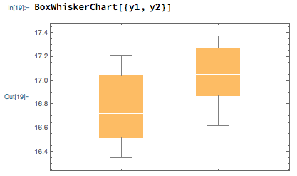
In[4]:= y1={16.85,16.40,...,16.59,16.57}
Out[4]= {16.85,16.4,...,16.59,16.57}
In[5]:= y2={16.62,16.75,...,17.08,17.27}
Out[5]= {16.62,16.75,...,17.08,17.27}
In[46]:= TTest[{y1,y2},Automatic, "TestData"]
Out[46]= {-2.18688,0.0421967}
In[48]:= Mean[y1]-Mean[y2]
Out[48]= -0.278
In[65]:= TTest[{y1,y2},0]
Out[65]= 0.0421967
In[69]:= MeanDifferenceCI[y1,y2]
Out[69]= {-0.546174,-0.00982586}
In[68]:= MeanDifferenceCI[y1,y2,EqualVariances->True]
Out[68]= {-0.545073,-0.0109266}
Appendix: R Code
References
- ↑ Wikipedia. 2019. WikipediA: the Free Encyclopedia. Retrieved from wikipedia:Design of experiments.
- ↑ 2.0 2.1 2.2 Douglas C. Montgomery. 2013. Design and Analysis of Experiments (8th. ed.). Wiley, New York, NY.
- ↑ Wikipedia. 2019. WikipediA: the Free Encyclopedia. Retrieved from wikipedia:List of statistical software.


